 Ben
Ben So we’re back with more Statistical Learning. In this class, we introduce the idea of regularization and some of the statistical underpinnings there.
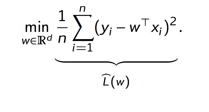
In the last class, Lorenzo made reference to how OLS regression is basically a learning algorithm to explore the space of possible linear functions that may minimize the “risk” of using a model’s prediction (\(\hat{Y}\)) versus the actual value. With OLS, risk minimization looks like this:
This shouldn’t look too strange to anyone who’s worked with OLS regressions before. Neither should the equation for finding the minimizer of \(w\):
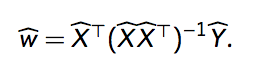
I don’t feel equipped to derive this right now, but check out this source for a good walkthrough of getting to this point (and beyond).
The first part of this minimizer (everything except the \(\hat{Y}\)) is called the pseudoinverse. The only reason I mention this is because after some magic, Lorenzo incorporates the Singular Value Decomposition (SVD) of \(X\) to go from \(w\) to the pseudoinverse of \(w\) (\(\hat{w}^\dagger\)).
Brief aside on SVD: Basically you’re decomposing the matrix X into three matrices, U, S and V, which capture how the data are aligned in space. S, in this case, is the singular values, and captures what could be considered the “importance” of a particular vector (from U or V) in the decomposition.
Why reformulate it like this? Lorenzo explains that this shows how OLS by design tends to cleave towards principal components. I was really hoping to have a pithy summary of why this is, but I really didn’t understand very well. I think this formulation is more useful when used in conjunction with the idea of “regularization”.
Regularization, briefly, is adjusting the parameters of a model to account for inherent noise in the data. We covered this a bit in the last class, that the goal of ML is to minimize the “risk” of using the model’s predictions over the reality. You can imagine to do that effectively we’d need to ensure we don’t create a model that performs well only on the dataset we have (i.e. keep an eye on the “generalizability”).
Lorenzo introduces one method for implementing regularization; Ridge Regression. That means adding the L2-norm of the weight vector to the ERM formulation:
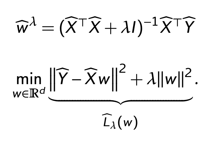
Note the lambda, which corresponds to the regularization strength. With lambda involved, the SVD formulation looks like this (more math magic):
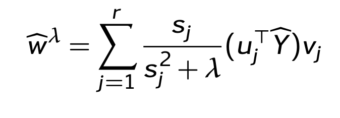
In this case, you can see how when s is greater than lambda, we get back to our original SVD formulation. When lambda is greater than s, then the first term becomes 1/lambda, which will shrink the size of \(w\). So, for components that are more “important”, the weights are mostly unaffected by lambda, but for components that aren’t very important, lambda will shrink them.
I find this idea a really neat, intuitive explanation of how regularization works, mathematically. We’ll be revisiting this in later lectures, but I thought it was important to tease this out as the main point of this lecture.
Again, I struggle a bit to understand why un-regularized OLS is naturally inclined towards principal components. Maybe I’ll write more on this later. In the meantime, if you have a good way of explaining this, or if you want to discuss, let me know!