 Ben
Ben Now we’re getting into the meat of things. This lecture was taught by Kian Katanforoosh and dove into a set of examples of Deep Learning projects to discuss design considerations. I’ll walk through some of this. Again, all images/material are from the course unless otherwise specified.
Kian started out with an overview of Neural Networks (NNs), generally. It was super high-level, but it covered the basics: An NN consists of a few main parts:
- Data: Kind of obvious, but considering what data to use for what problem is a key point in this lecture
- Architecture: This is the setup of the model and how it uses the parameters it learns
- Parameters: These are learned by the model, usually in the form of weights between nodes in the model architecture
- Hyperparameters: Prespecified parameters that govern the learning process (e.g. learning rate)
- Loss function: A big one, this is essentially how the parameters are learned. The model is trying to produce an output based on the input and the loss function is the measure of how “wrong” that output is. Based on that “wrongness”, the parameters are updated.
- Activation function: This translates the final layer of the network into the output. A simple one (and one Kian starts with) is the sigmoid activation function, which is used for assigning probabilities to two output classes.
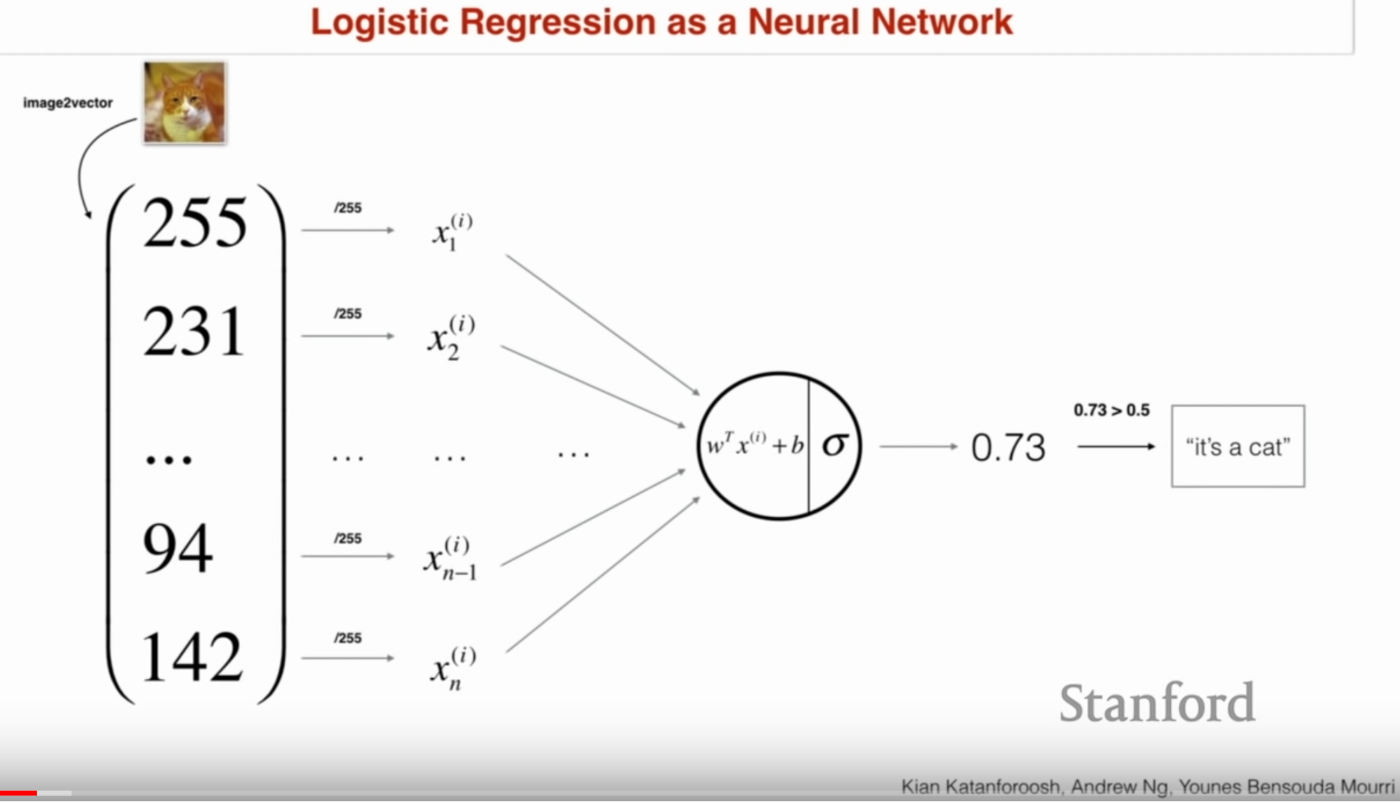
Above is Logistic Regression visualized as a NN. In this case, pixel intensities are passed as inputs to a model that learns weights to predict whether the image is a cat or not a cat. Kian expands this to a multi-class case (i.e. what type of animal is it) where the output would be a one-hot vector (i.e. one class marked positive out of multiple classes).
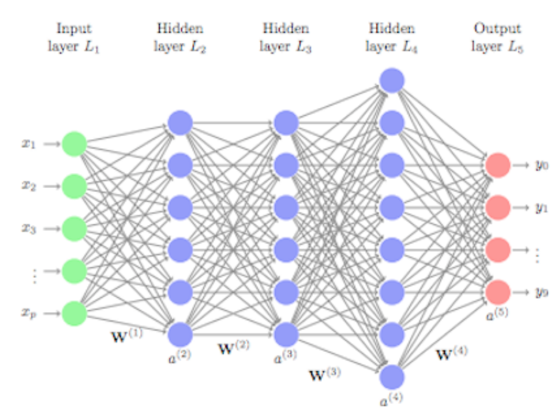
This example network is just single-layer, though. More complex architectures have many layers, which means looking something like this:
 http://uc-r.github.io/feedforward_DNN
Kian introduces notation for this type of network, which I think is worth putting here. It’s something I keep forgetting!
\[a_k^l\]Where node a is the kth neuron in layer l. So the first node in the first layer would be \(a_1^1\).
With the basics out of the way, Kian goes right into some pretty interesting examples, working with the audience to flesh out the needs of each use-case.
Day and Night Classification
Goal: Identify if an image is taken during the day or night
- Data
- If outdoor images, ~10k sample needed
- If the images are indoors, the task is much more complex and would require ~100k images
- Input
- Image pixels
- Resolution should be low, but not so low that human performance would be impacted
- Output: Binary, either day or night
- Architecture: Fully-connected shallow network
- Loss: Log-likelhood (kind of like standard logistic regression)
Face verification
Goal: Based on an image taken by a security camera, detect whether a person has access to a facility
- Data
- The image-ID database for the facility
- Potentially would need to be supplemented by other images of the person in front of a camera
- Input: The image the camera sees, at pretty high resolution for detail (412x412)
- Output: Binary, verified/not verified
- Architecture:
- Simple solution: Pixel to pixel comparison between ID image and camera image However, there’s likely to be pretty large distances, so it makes sense to compare the final layer encoding of the ID image and the camera image when run through the network
- For this purpose, likely enough to use an existing pretrained image network
- Loss
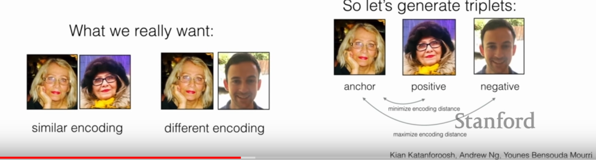
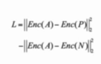
- Triplet loss: Minimize the distance between images of the same person and maximize distance between images of different person
- In this case, this means manufacturing a triplet dataset
Face recognition
Goal: Identify who the security camera is seeing
- Data, Input, Architecture: Same as above
- Output: Identify of person at camera
- Loss
- In this case we want to accurately predict who is in front of the camera
- For this purpose, we would use the network’s encoding and use something like K-Nearest Neighbors to identify the person
Art generation
Goal: Manipulate a content image to match a certain art style
- Data/Input: Any content + style image
- Output: Content image in given style
- Architecture:
- Again can use pretrained image network
- The earlier layers typically extract more basic features (e.g. edges), so can use that encoding to get “content”
- Style: Kian doesn’t go into detail here, but says there’s an technique called a “Gram Matrix” that’s particularly equipped for encoding “style”
- Loss
- Minimize the distance between the output’s style and content and the style/content encodings
This is a really interesting example because you’re not training the network and it doesn’t matter what image you put into the network. You could start with white noise, but because the network is trying to create an output that has both style and content components, after a few epochs, the image output will look like a fusion between the two.
Trigger word detection
Goal: Identify from a 10-sec audio clip whether a “trigger word” was said
- Data
- Need a lot here to account for so much variation
- These samples should be distributed across accents, kids/adults, etc
- Input: 10-sec clips with sample rate chosen based on human performance
- Output
- Can use 0/1 for the full 10-sec clip, but might make sense to have 0/1 for each time-step
- May also make sense to have the training dataset have all “1” after the trigger word was detected to deal with imbalance
- Architecture: Recurrent Neural Network
- Loss: Sequential log-loss
Kian notes that the main issue here is that there needs to be some strategy behind data manufacture. It may make sense to create 10-sec clips out of a combination of trigger words, non-trigger words and background noise. This way you can create a ton of samples, and you have simulated a real-world dataset (i.e. one that has noise and words).
I thought this lecture was really dense and super informative. I do wish there was a bit more time spent on some of the examples, as I think glossing over elements made the whole example a bit confusing. For example, I didn’t really understand the style extraction strategy for the art generation example. Kian mentioned a “Gram Matrix”, but didn’t go into it. I looked up Gram Matrices in the context of style transfer and turned up this pretty good explanation.
Because every column is multiplied with every row in the matrix, we can think of the spatial information that was contained in the original representations to have been “distributed”. The Gram matrix instead contains non-localized information about the image, such as texture, shapes, and weights — style!
This makes intuitive sense to me, but I wish it was explained as part of the example.
See you next time!